pt(2.5, nrow(UScereal)-(3+1), lower.tail = FALSE)[1] 0.007562028So you fit a model and all of your residuals are within \(\pm 1\). That’s great! Isn’t it? Well it all depends on the scale of the data you’re working with. If you are trying to model the weight of adults based on waist circumference than being consistently within \(\pm 1\) lb would be great. If instead you are trying to predict a student’s blood alcohol level based on the number of beers they’ve had a \(\pm 1\) error is pretty lousy since no one has a blood alcohol over 1 (or even 0.5).
Simply put, studentized residuals are a standardized residual measure to help you assess the size of the errors without needing to know detail around the context of the data. A studentized residual is obtained by dividing the raw residual by an estimate of its standard deviation. What is the estimate of its standard deviation? Refer back to Equation 7.3 in Chapter 7 and you’ll see this is something we’ve already worked with and \(H\), the hat matrix, plays a key role.
The studentized residual for the \(i\)th observation is given by:
\[t_i = \frac{e_i}{\sigma \sqrt{(1-h_{ii})}} \]
where:
Fundamentally, this approach is no different than the z-score formula you likely saw in intro statistics or the test-statistic format you’ve seen in basic hypothesis testing. The \(t_i\) studentized residual is just the observed error, minus the expected error which is always zero by design, then divided by a standard error.
So now that you have studentized residuals what can you do with them? Their main use is in being able to quickly identify outlier observations and have a consistent scale in which to think of just how much of an outlier they actually are. An outlier point with a studentized residual of 2-3 isn’t too bad, but an studentized residual of 17 is worth a look no matter what the scale of your y variable is.
To get the studentized residuals for a fitted model you can use the rstudent function contained in the stats library. The example here explores calorie content of cereals from the UScereal data set in the MASS library.
model_cereal<-lm(calories~fat+sugars+carbo, data=UScereal)
stud.res<-rstudent(model_cereal)

hist(model_cereal$residuals, main="", xlab="Observed Residuals", breaks=8)
hist(stud.res, main="", xlab="Studentized Residuals", breaks=8)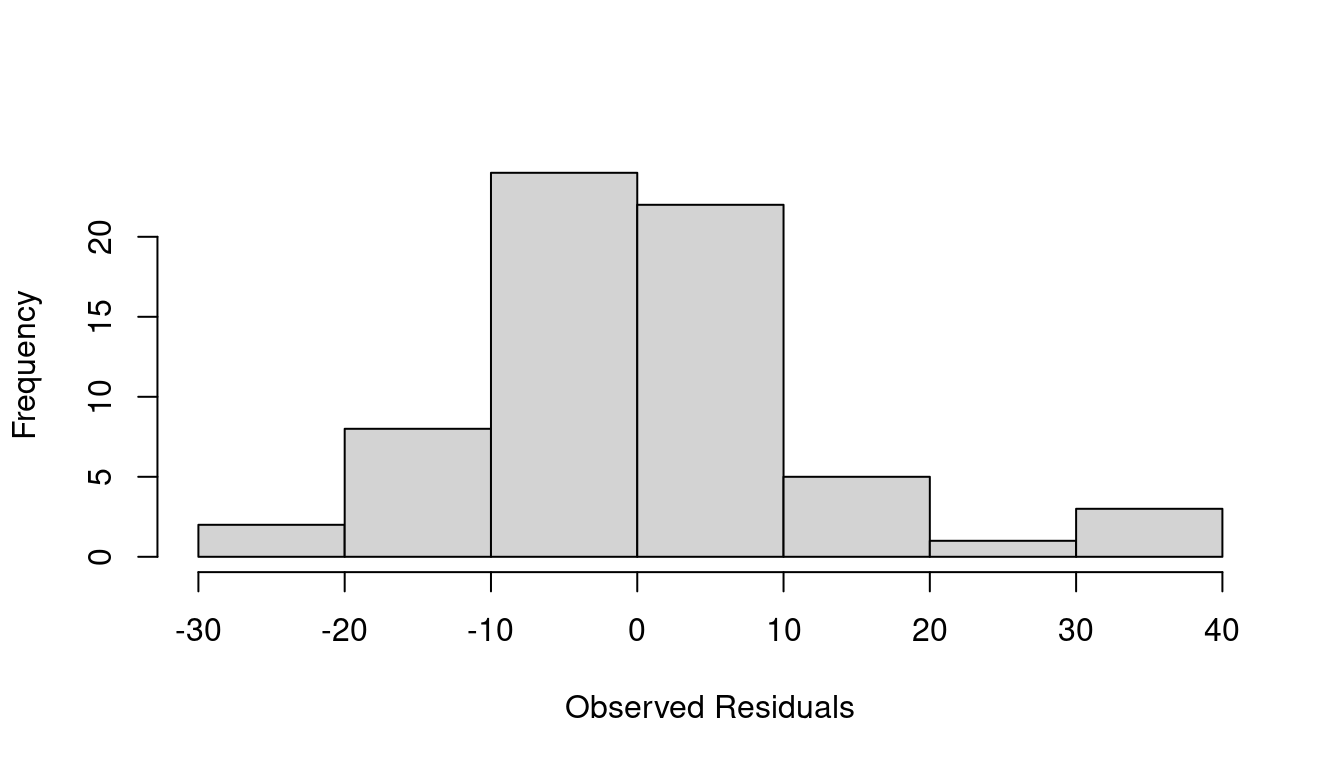
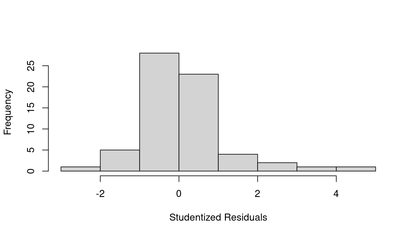
A summary of studentized residuals shows the most extreme outlying point has \(t_i=4.654\) which is definitely worth a second look. You can refer to a Student’s t-distribution with \(n-(p+1)\) degrees of freedom and see that a residual even 2.5 or larger should only happen about 0.76% of the time.
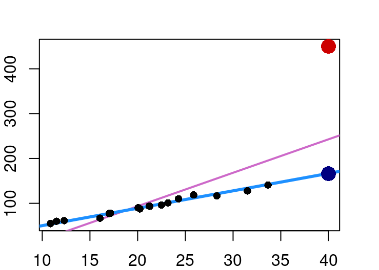
pt(2.5, nrow(UScereal)-(3+1), lower.tail = FALSE)[1] 0.007562028Outlier points in regression are not necessarily a problem. Where problems do occur is when the outlier is in a position that causes it to have undue influence over the regression fit. Consider Figure 9.2 below with two distinct outliers on the far right both at an x-value of 40.
In the case of the navy outlier point, it is far removed from the typical x values, but lies on the same x-y line that seems to fit the non-outlier points so it doesn’t exert an unusual amount of influence on the blue line fit.
The red outlier point however lies much higher than the linear pattern of non-outliers would expect. Because of this, inclusion of that one point when fitting the model moves the line from the blue fit to the one shown in orchid.
To identify outlier points that might be influential, you can use the leverage metric. The leverage for a point is simply that point’s corresponding diagonal element of the “hat matrix”. On average, leverage will be about \((p+1)/n\), and any point with a leverage greater than 2.5 times that is worth a closer look.
Another popular diagnostic metric to assess when a point might be unduly influential is Cook’s Distance. Cook’s distance combines information from both the residual size and the leverage and is defined as:
\[ D_i = \frac{e_{i}^2}{(p+1) \hat\sigma^2} \times \frac{h_{ii}}{(1-h_{ii})^2} =\frac{t_i^2}{p+1}\times\frac{h_{ii}}{1-h_{ii}} \]
where:
This highlights that Cook’s distance increases if an observation has a high studentized residual, has a high leverage, or both. A rule of thumb is to examine points with \(D_i > 4/n\), where \(n\) is the total number of observations. Ultimately though, any value that stands out from most others is worthy of a closer inspection.
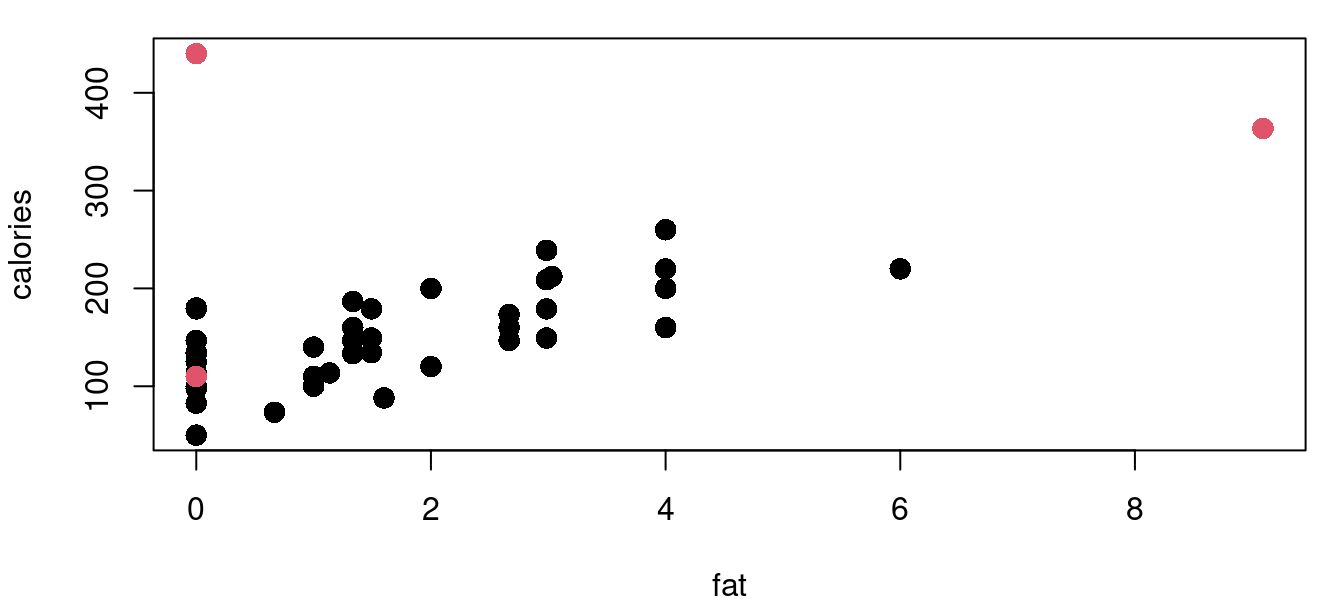
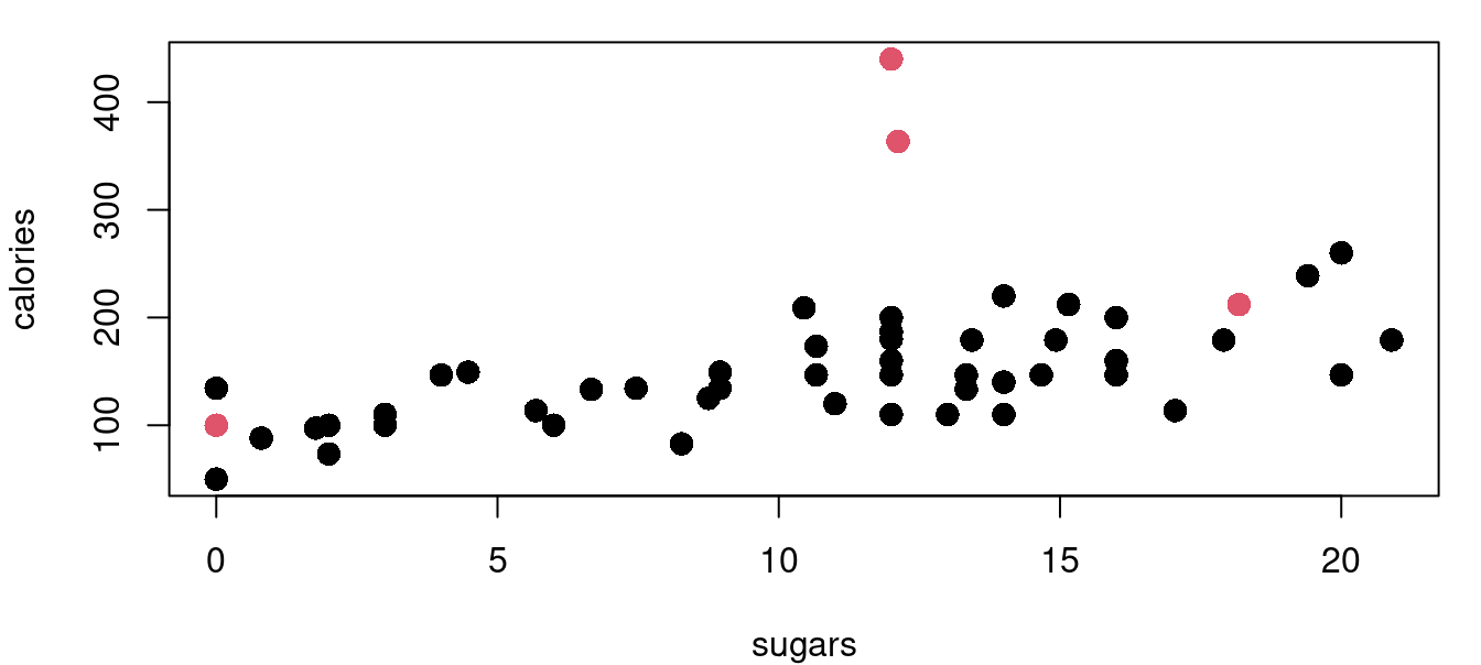
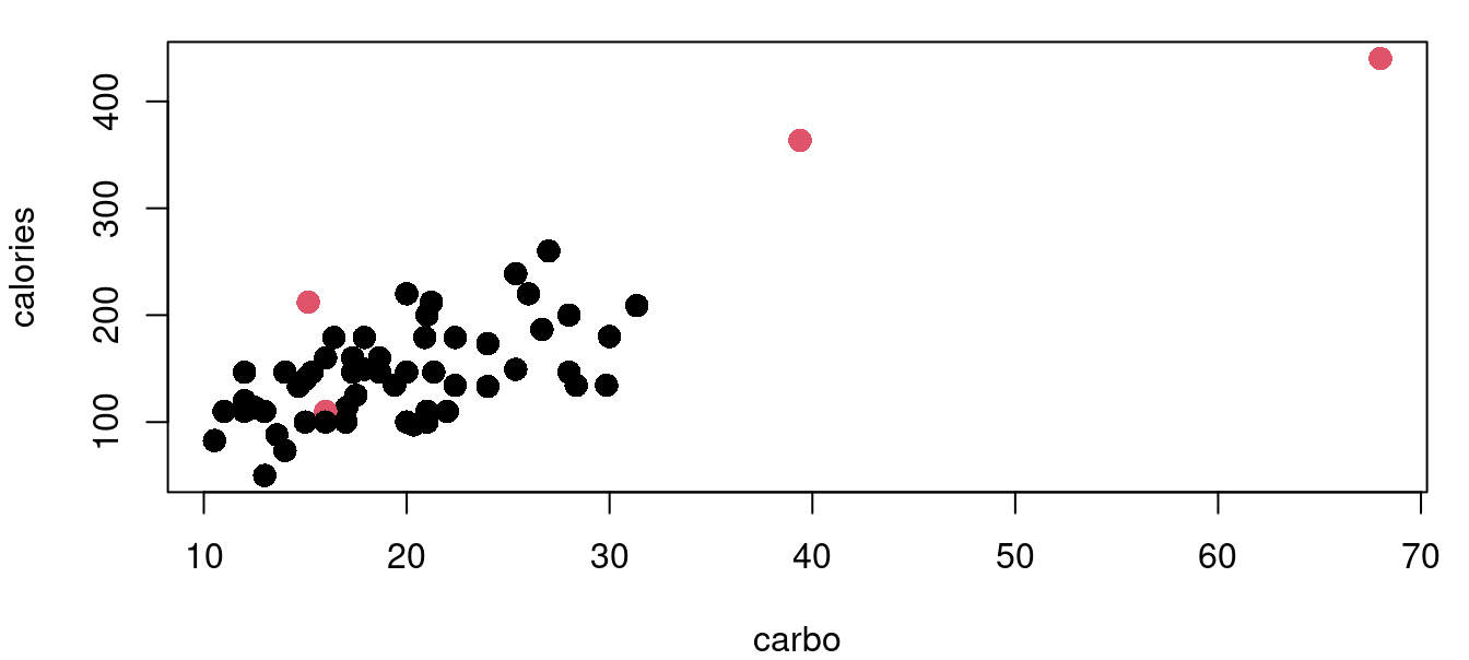
The functions for leverage and Cook’s distance are built into the stats library that loads by default. Continuing with the cereal nutrition example we find that there are three points with high leverage values.
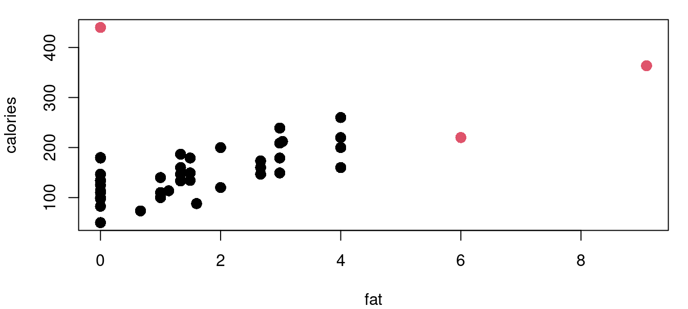
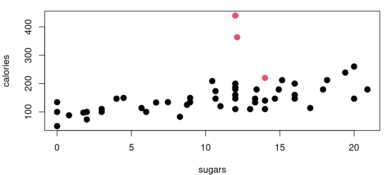
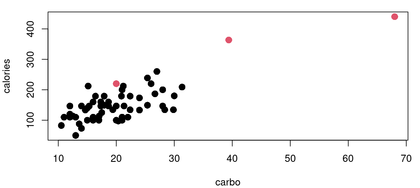
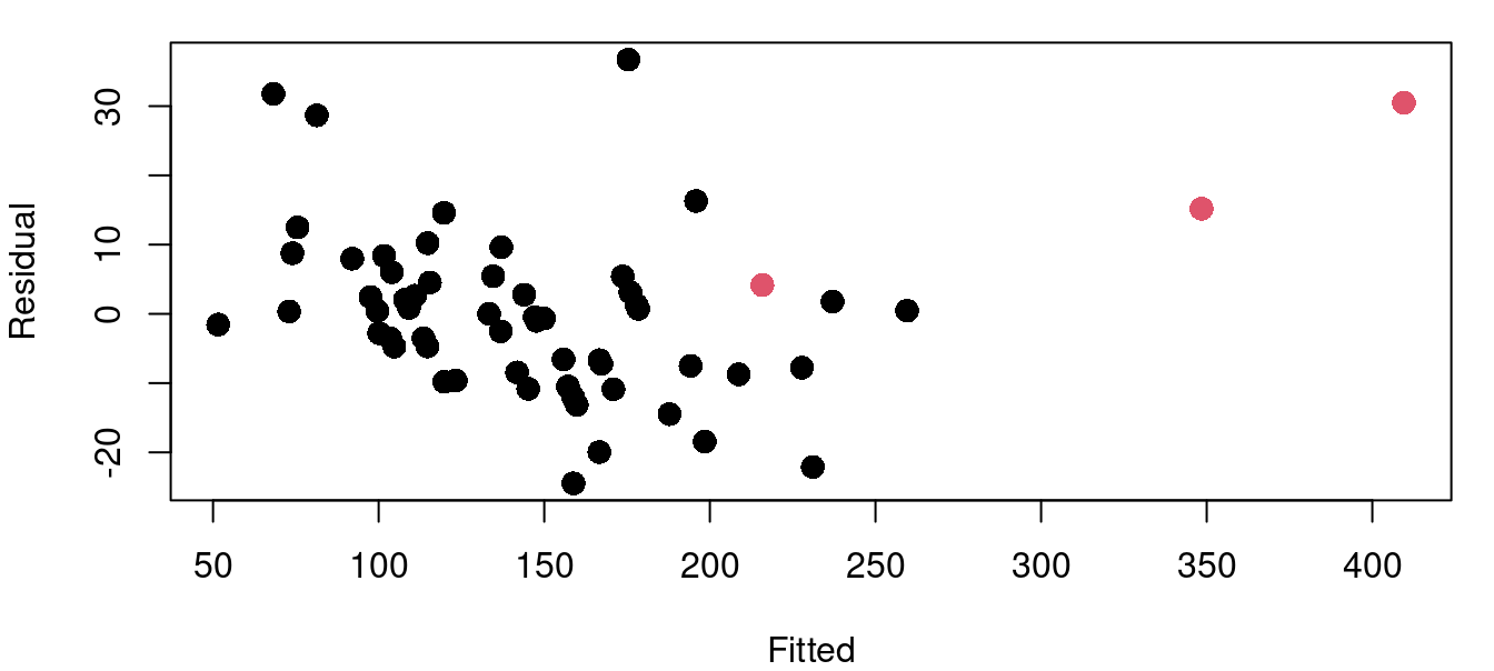
The hatvalues function returns the hat matrix diagonal for a fitted model object. From there it is a simple task to identify those that exceed our threshold of two and a half times \((p+1)/n\). Figure 9.3 above shows four plots of the cereal data with high leverage points marked in red. Leverage calculations are shown below.
model_cereal<-lm(calories~fat+sugars+carbo, data=UScereal)

lev_cereal<-hatvalues(model_cereal)
((2+1)/nrow(UScereal))*2.5
[1] 0.1153846sort(lev_cereal, decreasing=TRUE)[1:6] Grape-Nuts Great Grains Pecan Cracklin' Oat Bran
0.61399054 0.42563479 0.14574239
Fruitful Bran Shredded Wheat spoon size Oatmeal Raisin Crisp
0.08625599 0.08324148 0.08255166 The process is similar for calculating Cook’s distance. There are four cereals flagged with the Cook’s distance metric with Grape-Nuts becoming identified as a very significant standout with a \(D_i>6\). Here in Figure 9.4 are the same four cereal plots with red points indicating those with a Cook’s distance greater than the \(4/n\) threshold.
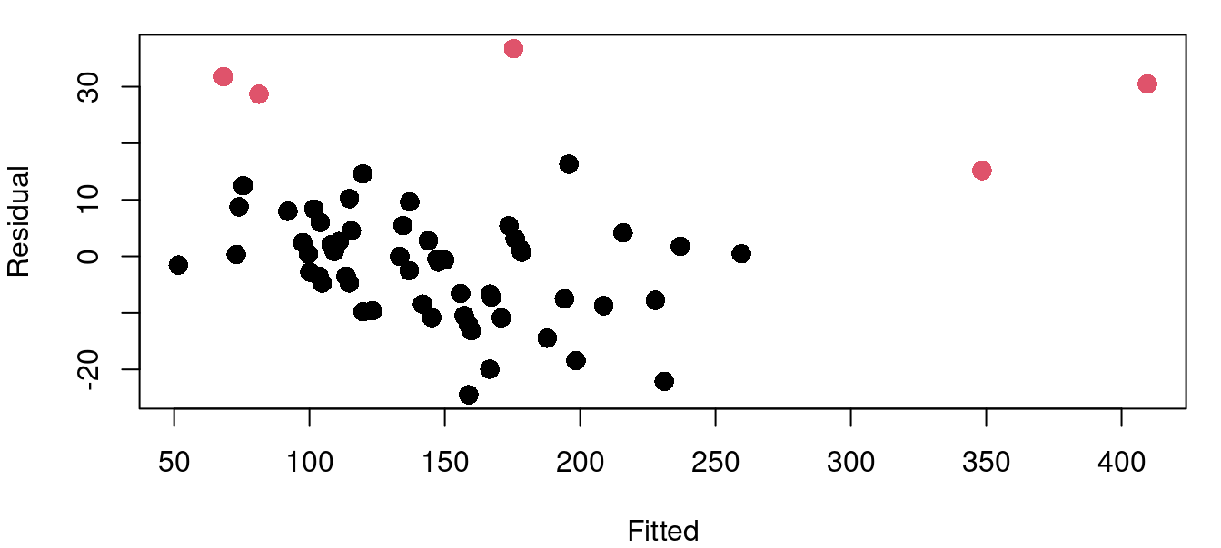
Below shows using the cooks.distance function, and a listing of the top six values.
cd_cereal<-cooks.distance(model_cereal)
4/nrow(UScereal)
[1] 0.06153846sort(cd_cereal, decreasing=TRUE)[1:6] Grape-Nuts Great Grains Pecan 100% Bran
6.43414435 0.50046528 0.13898120
All-Bran with Extra Fiber Special K Nutri-Grain Almond-Raisin
0.12924058 0.06608620 0.04776351 To understand the exact influence yielded by a row of your data, DFFits and DFBetas are used. DFFits will tell you how the fit of your model changes with the inclusion and exclusion of each point. DFBetas tells you how the estimated \(\hat\beta\) parameters change with the inclusion and exclusion of each point.
For example, in our calories~fat+sugars+carbo model in the UScereal data frame, the DFFit for Cinnamon Toast Crunch is -0.237. That means that when the model is fit including Cinnamon Toast Crunch (CTC) in the training set, the fitted value for CTC is 0.237\(\sigma_{CTC}\) lower than when the model is fit excluding CTC from the training set. Note that it is in units of \(\sigma\) specific to the CTC observation, not the broader \(\sigma\) of the model. In general, the formula for DFFits for observation \(i\) is:
\[ DFFits_i=\frac {\hat y_i - \hat y_{(i)i}}{\sqrt{\hat\sigma_{(i)}^2h_{ii}}} \]
where:
DFBetas is the same idea, but looking at the difference in \(\beta\) values with and without each observation rather than at the difference in fits.
\[ DFBetas_j=\frac{\hat\beta_j - \hat \beta_{j(i)}}{\sqrt{\hat\sigma^2_{j(i)}(X^TX)^{-1}_{jj}}} \]
where:
You can refer back to Chapter 7 to review the derivation of \(\hat\sigma^2(X^TX)^{-1}\) as the variance matrix for the \(\beta\) vector.
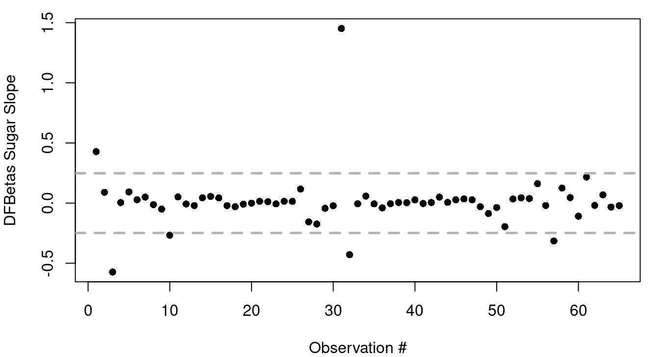
Simple plots of DFfits and DFBetas are often helpful in spotting influential observations. An example of this is in Figure 9.5. As a general rule, DFfits values greater than \(2\sqrt{p/n}\) or less than \(-2\sqrt{p/n}\) are worthy of a second look so reference lines have been included in Figure 9.5 (a) to show those thresholds. For Figure 9.5 (b) reference lines are included at \(\pm 2/\sqrt{n}\), the general rule of thumb for evaluating DFBetas.
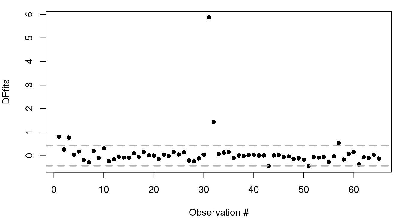
Here are the series of steps to calculate out the DFFits value of Cinnamon Toast Crunch, the \(11^{th}\) row of USCereals, in R.
mod_cereal<-lm(calories~fat+sugars+carbo, data=UScereal)
fit1<-mod_cereal$fitted.values[11]

mod_noCTC<-lm(calories~fat+sugars+carbo, data=UScereal[-11,])
fit2<-predict(mod_noCTC, UScereal[11,])

CTC_hat<-hatvalues(mod_cereal)[11]
CTC_sig<-sqrt(summary(mod_noCTC)$sigma^2 * CTC_hat)

(fit1-fit2)/CTC_sig
Cinnamon Toast Crunch
-0.2372347 The easier way is to use the dffits function that is part of the stats library in R. The only input needed is the fitted model object, and DFFits for all observations will be returned.
mod_cereal<-lm(calories~fat+sugars+carbo, data=UScereal)
dfs<-dffits(mod_cereal)
dfs[11]
Cinnamon Toast Crunch
-0.2372347 For DFBetas, here is the DFBeta for the sugars slope considering the Cinnamon Toast Crunch row of data.
  mod_cereal<-lm(calories~fat+sugars+carbo, data=UScereal)
  fit1<-mod_cereal$coef[3]

  mod_noCTC<-lm(calories~fat+sugars+carbo, data=UScereal[-11,])
  fit2<-mod_noCTC$coef[3]

  sig1<-summary(mod_noCTC)$sigma^2

  xmat<-as.matrix(cbind(rep(1, 65), UScereal[,c(4,7,8)]))
  inv<-solve(t(xmat)%*%xmat)
  siguse<-sqrt(sig1*inv[3,3])

  (fit1-fit2)/siguse
sugars
0.08030943 To do this automatically in R you can use the dfbetas function. The dfbetas function returns a full matrix of values with each row corresponding to an observation, and each column corresponding to a different \(\beta\). For the sugar slope change associated with omitting Cinnamon Toast Crunch we’ll want the \(11^{th}\) row and the \(3^{rd}\) column.
dfb<-dfbetas(mod_cereal)
dfb[11,]
(Intercept) fat sugars carbo
-0.06653261 -0.19889228 0.05119340 0.07823310 Be aware that in addition to the dfbetas function, there is also a dfbeta function. The dfbeta function without the trailing s, provides the raw difference in \(\beta\) fits without scaling by the standard error of \(\beta\). This can also be useful sometimes, but it is important to know which one you’re looking at.
dfb_raw<-dfbeta(mod_cereal)
dfb_raw[11,]
(Intercept) fat sugars carbo
-0.32113477 -0.20768424 0.01484826 0.01446437